Work transfer for open system

First law of Thermodynamics is based on Energy conservation . In the previous post we studied about two forms of thermodynamics .

In first law of Thermodynamics for open system we described the relation,

m{ h₁ + v₁ ² /2 + gZ₁ } + ∆Q/∆t = m{ h₂ + v₂ ² /2 + gZ_{2} +} ∆W/∆t

This relation is Steady Flow Energy Equation or SFEE.

With the help of this equation , we can find out the value of work transfer for open system.

Let’s assume the kinetic energy and potential energy negligible

Now from SFEE ,

m{ h₁ + v₁ ² /2 + gZ₁ } + ∆Q/∆t = m{ h₂ + v₂ ² /2 + gZ_{2} +} ∆W/∆t

then ,

mh₁ + ∆Q/∆t = mh₂ + ∆W/∆t

∆Q/∆t = m (h₂ – h₁) + ∆W/∆t

∆Q/∆t = m dh + ∆W/∆t

Now , considering it for per unit mass

Then ,

∆Q/m = dh + ∆W/∆m______________eq(1)

we know that ,

∆Q = dH – VdP , where V = Total volume

Dividing this relationship by ∆m

∆Q/∆m = dH/∆m – VdP/∆m

Here , dH/∆m = dh = specific enthalpy

& , V/∆m = v = specific volume

So ,

∆Q = dh – vdP__________eq(2)

Comparing eqn (1) and(2)

We get ,

∆W/∆m = – int(vdP)

This is the work transfer for open system .

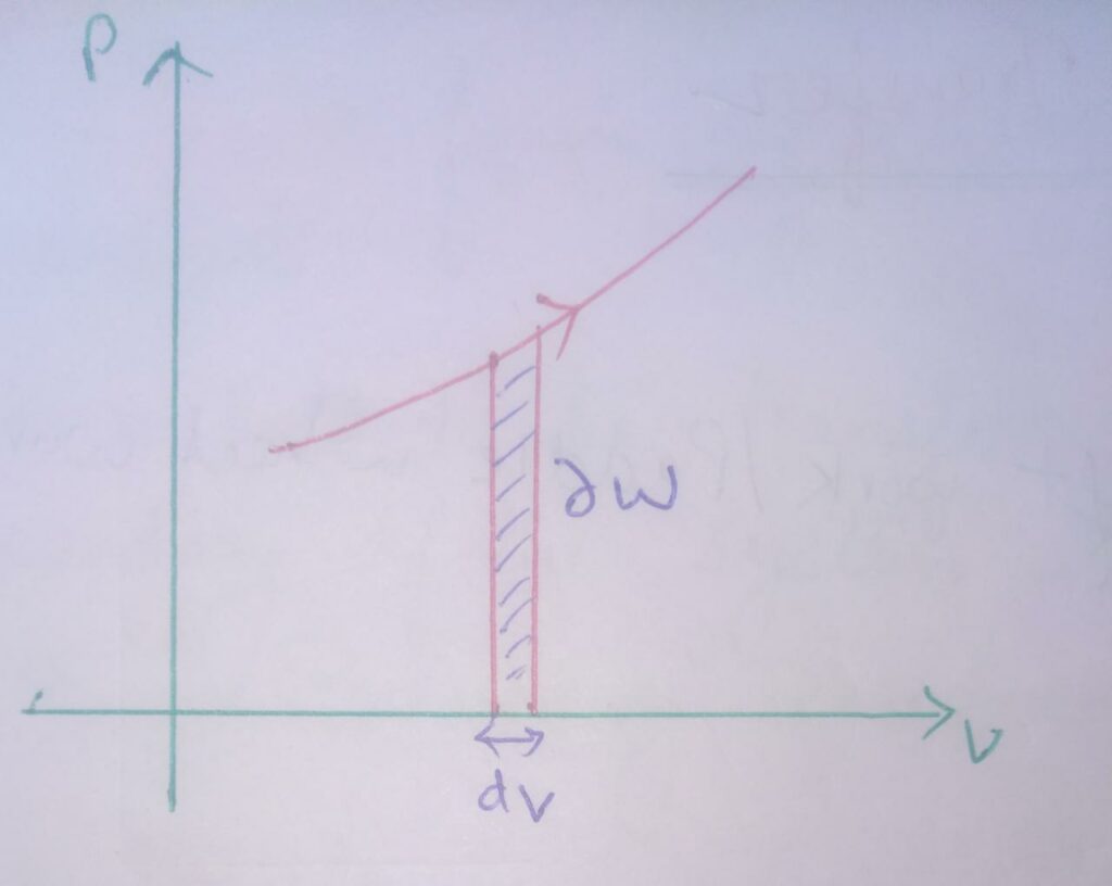
Graphical representation of work transfer for open system :

For open system :

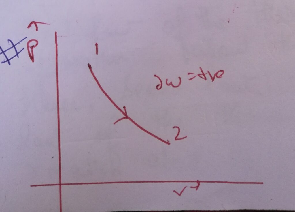
Case (I) :

∆W= – int( vdP) , where dP = +ve

∆W=-ve ,

Then graphically it is represented as –

Here the slope of the PV curve is increasing .

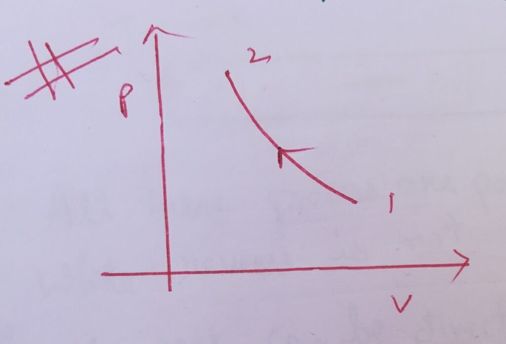
Case (II) :

∆W= – int( vdP) , where dP = -ve

∆W = +ve

Then graphically it is represented as –

Here the slope of the PV curve is decreasing .

Graphical representation of work transfer for closed system :

∆W = PdV , here dV = -ve

Therefore , ∆W = -ve

•